[Paper Review] DDPM(Denoising Diffusion Probabilistic Models)
DDPM
- Paper: Denoising Diffusion Probabilistic Models ; arxiv
Diffusion Process는 Markov Chain과 Gaussian distribution을 기반으로 image로 부터 noise를 더해가는 과정인 Diffusion process와 이 process를 보고 학습을 통해 noise로 부터 이미지를 생성해내는 denoising process로 이루어져 있다. DDPM 모델은 학습 파라미터들을 부분적으로 상수로 정의함으로써 그 수를 줄여 모델 학습 과정을 단순화하여 Diffusion Model 발전의 시초가 된 모델이다. DDPM 논문의 핵심은 neural network로 표현되는 p 모델이 q를 보고 noise를 걷어내는 과정을 학습하는 것이다.
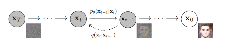
Diffusion Process (Forward Process)
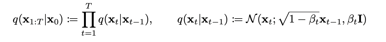
$ q(X_{1:T}|X_{0}) $ : q는 이미지로부터 noise를 주입하는 과정으로 Markov Chain에 따라 0 step부터 T step까지 $\beta_{t}$를 이용하여 확률분포로 나타내었다. $\beta_{t}$는 Beta scheduling(Cosine Scheduling이 가장 성능이 좋다고 한다)을 이용하여 미리 constant하게 정해놓았기에 Diffusion Process에서는 trainable parameter가 없다. Diffusion Process는 Denoising Process를 진행하는 Network의 본보기로 사용되는 것이다.
$ q(X_{t}|X_{t-1}) $ : $X_{t-1}$의 mean $ \mu_{t-1} $, std $ \sigma_{t-1} $ 을 알고 있을 때 $X_{t}$에 대한 확률분포이다. $X_{t-1}$은 Gaussian 분포를 띠기에, $X_{t-1}$를 나타내기 위해서는 $ \mu_{t-1} $, $ \sigma_{t-1} $를 알면된다.
$X_{t-1}$의 mean $ \mu_{t-1} $, std $ \sigma_{t-1} $ 을 알고 있을 때 $X_{t}$의 mean과 std는 다음과 같다.
$ \mu_{t} $ = $\sqrt{1-\beta_{t}} X_{t-1}$, $ \sigma_{t} $ = $ \beta_{t}$
$X_{t}$는 $ \mu_{t} $와 $ \sigma_{t} $로 표현되는 Gaussian 분포에서 샘플링한 결과이지만 Backpropagation을 위해 VAE(Various Autoencoder)에서 사용된 기법인 Reparameterization Trick
($X_{t}$ = $ \mu_{t-1} $ + $ \sigma_{t-1}$$\epsilon$ )을 이용하면 다음과 같이 나타낼 수 있다.
$X_{t}$ = $\sqrt{1-\beta_{t}} X_{t-1}$ + $ \sqrt{\beta_{t}}$$\epsilon$
=> Diffusion process를 보고 어떻게 Denoising network p가 denoising process가 되게 학습시킬 수 있을까? 이것이 DDPM의 핵심이다!
Denoising Process (Reverse Process)

Denoising Process의 과정은 $p_{\theta}(X_{t-1}|X_{t})$로 나타낼 수 있다. Denoising network p는 Forward Process q를 통해 학습하는데 상식적으로는 $q(X_{t-1}|X_{t})$를 학습한다고 판단할 수 있다. 하지만 $q(X_{t}|X_{t-1})$을 통해 $q(X_{t-1}|X_{t})$을 알수는 없다. 그렇다면 Denoising Network는 어떤 방식으로 학습을 진행해야 할까?
Denoising Network p가 나타내는 확률분포로 부터 원본 이미지 $X_{0}$가 나올 Likelihood가 최대가 되도록 만들면된다. 즉, $p_{\theta}(X_{0})$의 log-likelihood가 최대 혹은 Negative log-likelihhod가 최소가 되도록 학습이 이루어지면 된다. 식으로 표현하면 다음과 같다.
$\underset{\theta}{argmax}$ $log(p_{\theta}(X_{0}))$ = $\underset{\theta}{argmin}$ $-log(p_{\theta}(X_{0}))$
하지만 Denoising Network p는 $q(X_{t-1}|X_{t})$를 모사하기 위해 설정한 것이므로 $log(p_{\theta}(X_{0}))$는 intractable하다! 그래서 바로 구하지 못하고 Evidence of Lower Bound (ELBO)를 이용하여 Network의 학습방향을 설정한다. KL-Divergence 값은 항상 0보다 크므로 $-log(p_{\theta}(X_{0}))$를 최소화하는 식은 아래 식의 (0)과 같다. (0)의 우변($Loss_{Diffusion}$)을 최소화하는 것이 Network의 학습 방향이 되며 $Loss_{Diffusion}$을 정리하기 위한 식의 변형 과정을 아래에 나타내었다. (0)의 식의 우변($Loss_{Diffusion}$)만 고려해서 정리하였다. 말도 안되게 기네요..
<$Loss_{Diffusion}$>
$-log(p_{\theta}(X_{0})) \le$ $ -log(p_{\theta}(X_{0})) + D_{KL}(q(X_{1:T}\|X_{0})\parallel p_{\theta}(X_{1:T}\|X_{0}))$ $\dots$ (0)
< Calculate Loss Function for Denoising Network >
$ -log(p_{\theta}(X_{0})) + D_{KL}(q(X_{1:T}|X_{0})\parallel p_{\theta}(X_{1:T}|X_{0}))$ $\dots$ (1)
| $D_{KL}(q(X_{1:T}|X_{0})\parallel p_{\theta}(X_{1:T}|X_{0})) = E_q[log \frac{q(X_{1:T}|X_{0})}{p_{\theta}(X_{1:T}|X_{0})}]$, $p_{\theta}(X_{1:T}|X_{0}) = \frac{p_{\theta}(X_{0:T})}{p_{\theta}(X_{0})}$이므로 식을 대입. |
| (1)는 | $ -log(p_{\theta}(X_{0})) + E_q[\frac{q_(X_{1:T}|X_{0})}{p_{\theta}(X_{0:T})}] + log(p_{\theta}(X_{0})) = E_q[\frac{q_(X_{1:T}|X_{0})}{p_{\theta}(X_{0:T})}]$ 로 정리된다. |
$E_q[ log \frac{q_(X_{1:T}|X_{0})}{p_{\theta}(X_{0:T})} ]$ $\dots$ (2)
| $ log \frac{q_(X_{1:T}|X_{0})}{p_{\theta}(X_{0:T})}= log \frac{\prod_{t=1}^{T} q(X_t|X_{t-1})}{p_{\theta}(X_T)\prod_{t=1}^{T}p_{\theta}(X_{t-1}|X_t)}=-log(p_{\theta}(X_T)) + log \frac{\prod_{t=1}^{T} q(X_t|X_{t-1})}{\prod_{t=1}^{T}p_{\theta}(X_{t-1}|X_t)}= -log(p_{\theta}(X_T)) + \sum_{t=1}^{T}log \frac{q(X_t|X_{t-1})}{p_{\theta}(X_{t-1}|X_t)} $ |
| $ = -log(p_{\theta}(X_T)) + \sum_{t=2}^{T}log \frac{q(X_t|X_{t-1})}{p_{\theta}(X_{t-1}|X_t)} + log \frac{q(X_1|X_0)}{p_{\theta}(X_0|X_1)}$ |
| By Bayes Rule, $q(X_t|X_{t-1}) = \frac{q(X_{t-1}|X_{t},X_{0}) q(X_{t-1}|X_{t},X_{0})}{q(X_{t-1}|X_0)}$ | => 위의 $\sum$ 내부의 $q(X_t|X_{t-1})$에 이 식을 대입. |
| (2)는 | $ E_q[ -log(p_{\theta}(X_T)) + \sum_{t=2}^{T}log \frac{q(X_{t-1}|X_{t},X_{0}) q(X_{t}|X_{0}) } {p_{\theta}(X_{t-1}|X_t) q(X_{t-1}|X_{0})} + log \frac{q(X_1|X_0)}{p_{\theta}(X_0|X_1)} ]$ | 이고, |
| $ E_q[ -log(p_{\theta}(X_T)) + \sum_{t=2}^{T}log \frac{q(X_{t-1}|X_{t},X_{0})} {p_{\theta}(X_{t-1}|X_t)} + \sum_{t=2}^{T}log \frac{q(X_{t}|X_{0}) } {q(X_{t-1}|X_{0})} + log \frac{q(X_1|X_0)}{p_{\theta}(X_0|X_1)} ]$ 로 정리된다. |
$ E_q[ -log(p_{\theta}(X_T)) $ + $ \sum_{t=2}^{T}log \frac{q(X_{t-1}|X_{t},X_{0})} {p_{\theta}(X_{t-1}|X_t)}$ + $ \sum_{t=2}^{T}log \frac{q(X_{t}|X_{0}) } {q(X_{t-1}|X_{0})}$ + $ log \frac{q(X_1|X_0)}{p_{\theta}(X_0|X_1)} ]$ $\dots$ (3)
[A] [B] [C] [D]
| $ [C] = log(\frac{q(X_2|X_0)}{q(X_1|X_0)} \times \frac{q(X_3|X_0)}{q(X_2|X_0)} \times \dots \times \frac{q(X_T|X_0)}{q(X_{T-1}|X_0)}) = log(\frac{q(X_T|X_0)}{q(X_1|X_0)})$ |
| $[C]+[D] = log(\frac{q(X_T|X_0)}{q(X_1|X_0)}) + log(\frac{q(X_1|X_0)}{p_{\theta}(X_0|X_1)}) = log(\frac{q(X_T|X_0)}{p_{\theta}(X_0|X_1)})$ |
$ E_q[ -log(p_{\theta}(X_T)) $ + $ \sum_{t=2}^{T}log \frac{q(X_{t-1}|X_{t},X_{0})} {p_{\theta}(X_{t-1}|X_t)}$ + $ log \frac{q(X_T|X_0)}{p_{\theta}(X_0|X_1)} ]$ $\dots$ (4)
[A] [B] [C] + [D]
| $ [A] + [C] + [D] = log\frac{q(X_T|X_0)}{p_{\theta}(X_T)} - log (p_{\theta}(X_0|X_1)) $ |
| 마지막으로 [A] + [B] + [C] + [D]를 정리해보면 다음과 같다. |
$ E_q[ log\frac{q(X_T|X_0)}{p_{\theta}(X_T)} + \sum_{t=2}^{T}log \frac{q(X_{t-1}|X_{t},X_{0})} {p_{\theta}(X_{t-1}|X_t)} - log (p_{\theta}(X_0|X_1)) ]$ $\dots$ (5)
| $ E_q[ log\frac{q(X_T|X_0)}{p_{\theta}(X_T)} ] = D_{KL}(q(X_T|X_{0})\parallel p_{\theta}(X_T))$ |
| $ E_q[ \sum_{t=2}^{T}log \frac{q(X_{t-1}|X_{t},X_{0})} {p_{\theta}(X_{t-1}|X_t)}] = \sum_{t=2}^{T}D_{KL}(q(X_{t-1}|X_{t},X_{0})\parallel p_{\theta}(X_{T-1} | X_T))$ |
| 따라서 $Loss_{Diffusion}$을 정리하면 다음과 같다. |
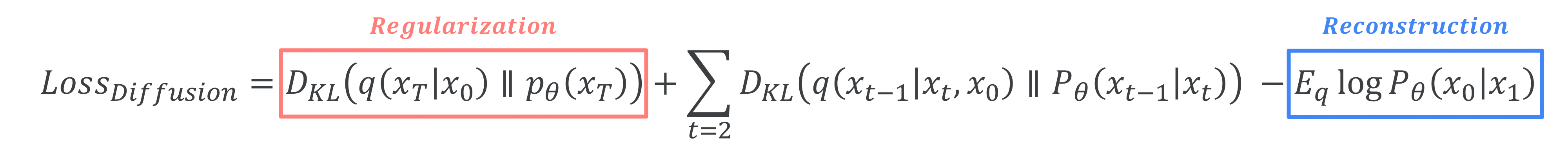
Regularization과 Reconstruction term은 Constant한 값으로 설정해도 영향이 없어서 Constant한 값으로 설정했다고 한다. 결국 DDPM에서 설정한 Denoising Network의 학습방향은 $q(X_{t-1}|X_t,X_0)$ 와 $p_{\theta}(X_{t-1}|X_t)$의 KL-Divergence값을 최소화하는 것이다. 즉, $q(X_{t-1}|X_t,X_0)$와 $p_{\theta}(X_{t-1}|X_t)$의 분포가 최대한 같도록 Denoising Network p가 학습하면 되는 것이다.
By Bayes Rule, $q(X_{t-1}|X_t, X_0) = q(X_t| X_{t-1})\frac{q(X_{t-1}|X_0)}{q(X_t|X_0)}$
=> Denoising Process를 Diffusion Process에 관한 식으로 나타낼 수 있다.
| $X_t = \sqrt{1-\beta_{t}} X_{t-1} + \sqrt{\beta_{t}}\epsilon = \sqrt{\alpha_{t}} X_{t-1} + \sqrt{1-\alpha_{t}}\epsilon$ | ($\alpha_t = 1 - \beta_t$) |
| Markov Chain 성질을 이용해 $X_{t-1}$을 $X_{t-2}$에 대해 나타내서 대입하고 $X_{t-2}$를 $X_{t-3}$에 대해서, 그리고 계속해서 $X_0$까지 나타낸다면 $X_t$는 다음과 같이 나타낼 수 있다. |
$X_t = \sqrt{\bar\alpha_{t}}X_0 + \sqrt{1-\bar\alpha_{t}}\epsilon$ ($\bar\alpha_{t} = \prod_{i=1}^{T}\alpha_i$)
$ \mu_{t} $와 $ \sigma_{t} $로 표현되는 Gaussian 분포에서 샘플링한 $X_t$를 우리는 Reparameterization Trick을 이용해 $X_{t}= \mu_{t} + \sigma_t \epsilon$ 로 나타냈음을 알기에 아래의 식들로 부터 $q(X_t| X_{t-1}), q(X_t| X_{0}), q(X_{t-1}| X_{0})$를 구할 수 있다.
$X_t = \sqrt{1-\beta_{t}} X_{t-1} + \sqrt{\beta_{t}}\epsilon$
===> $q(X_t|X_{t-1}) = N(\sqrt{\alpha_{t}}X_{t-1}, 1-\alpha_{t})$
$X_t = \sqrt{\bar\alpha_{t}}X_0 + \sqrt{1-\bar\alpha_{t}}\epsilon$ ($\bar\alpha_{t} = \prod_{i=1}^{T}\alpha_i$)
===> $q(X_t|X_{0}) = N(\sqrt{\bar\alpha_{t}}X_0, 1-\bar\alpha_{t})$
$X_{t-1} = \sqrt{\bar\alpha_{t-1}}X_0 + \sqrt{1-\bar\alpha_{t-1}}\epsilon$ => $q(X_{t-1}|X_0)$
===> $q(X_{t-1}|X_{0}) = N(\sqrt{\bar\alpha_{t-1}}X_0, 1-\bar\alpha_{t-1})$
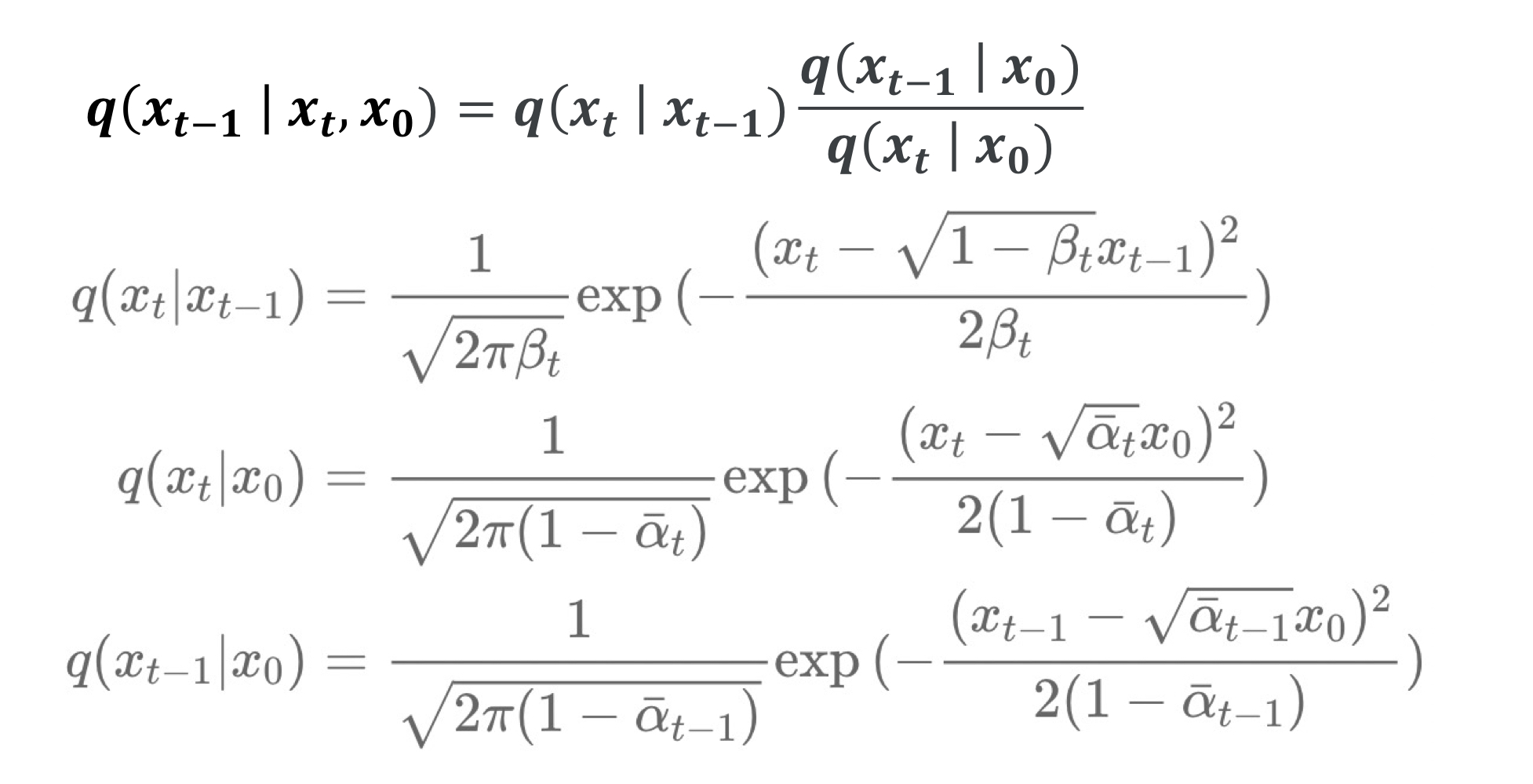
대입을 해보면 $q(X_{t-1}|X_t, X_0)$는 다음과 같이 나온다.
$q(X_{t-1}|X_t, X_0)$ = N($X_{t-1}$; $\frac{\sqrt{\bar\alpha_{t-1}}\beta_{t}}{1-\alpha_{t}}X_0 + \frac{\sqrt{\alpha_{t}}(1-\bar\alpha_{t-1})}{1-\bar\alpha_{t-1}}X_t$, $\beta_t$ $\frac{1-\bar\alpha_{t-1}}{1-\bar\alpha_{t}}$)
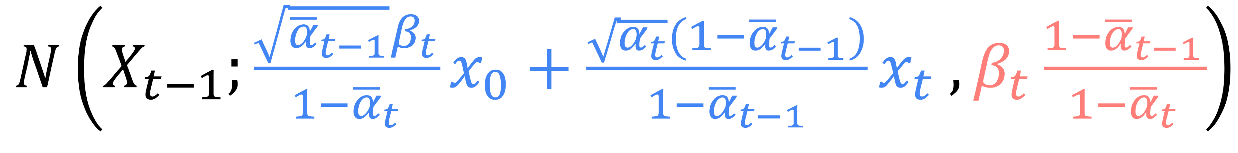
Variance는 우리가 알고 있는 값인 $\alpha, \beta$에 관한 식이므로 Network가 학습할 것이 없기에 $\tilde{\beta_{t}}$로 정의한다.
$X_t = \sqrt{\bar\alpha_{t}}X_0 + \sqrt{1-\bar\alpha_{t}}\epsilon$ ($\bar\alpha_{t} = \prod_{i=1}^{T}\alpha_i$)이므로 식을 정리하여 $X_0$에 대입하면 다음과같다.
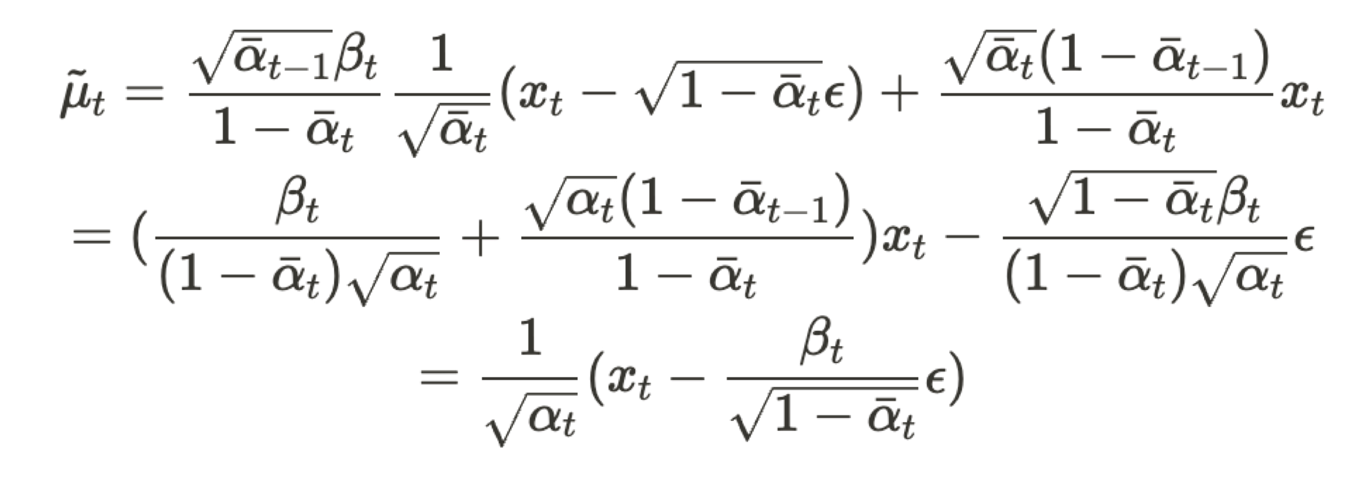
이때 Network가 학습해야 할 부분은 이미 알고 있는 값들을 제외하고 매 Step마다 빼주는 $\epsilon$이다. 따라서 Denoising Network p가 예측해야 하는 것은 $\epsilon_{\theta}(X_t)$라고 표현 가능하다.
- $ q_(X_{t-1}|X_t,X_0) = N(X_{t-1}; \frac{1}{\sqrt{\alpha_t}}(X_t - \frac{\beta_t}{\sqrt{1-\bar\alpha_t}}\epsilon), \tilde{\beta_{t}}$ )
- $ p_{\theta}(X_{t-1}|X_t) = N(X_{t-1}; \frac{1}{\sqrt{\alpha_t}}(X_t - \frac{\beta_t}{\sqrt{1-\bar\alpha_t}}\epsilon_{\theta}(X_t)), \tilde{\beta_{t}}$ )
$ q_(X_{t-1}|X_t,X_0) $와 $ p_{\theta}(X_{t-1}|X_t)$의 mean에 대해서 L2 Norm을 구하면 최종적으로 DDPM에서 간략화한 Denoising Network의 Loss식은 아래와 같이 정리된다.
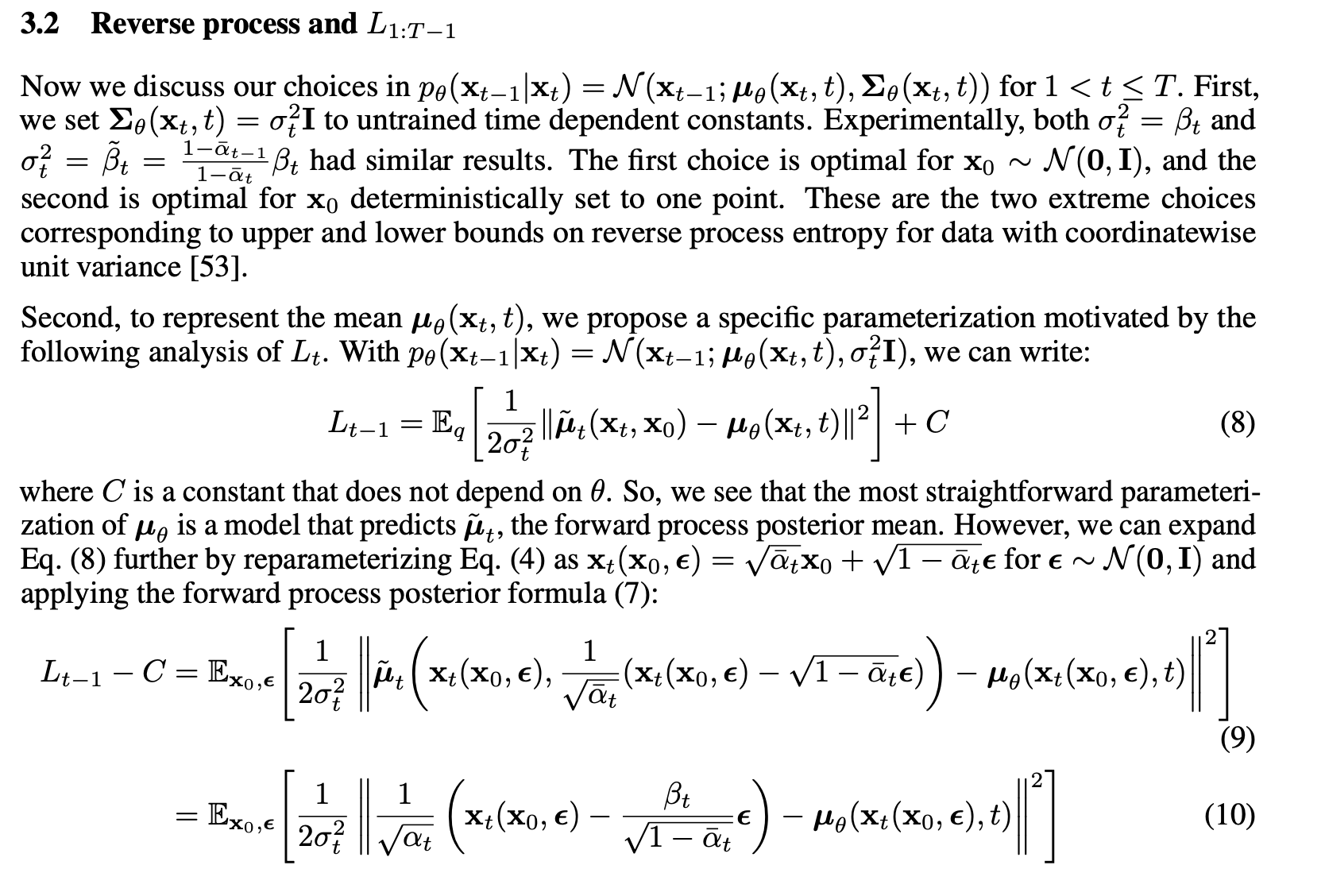
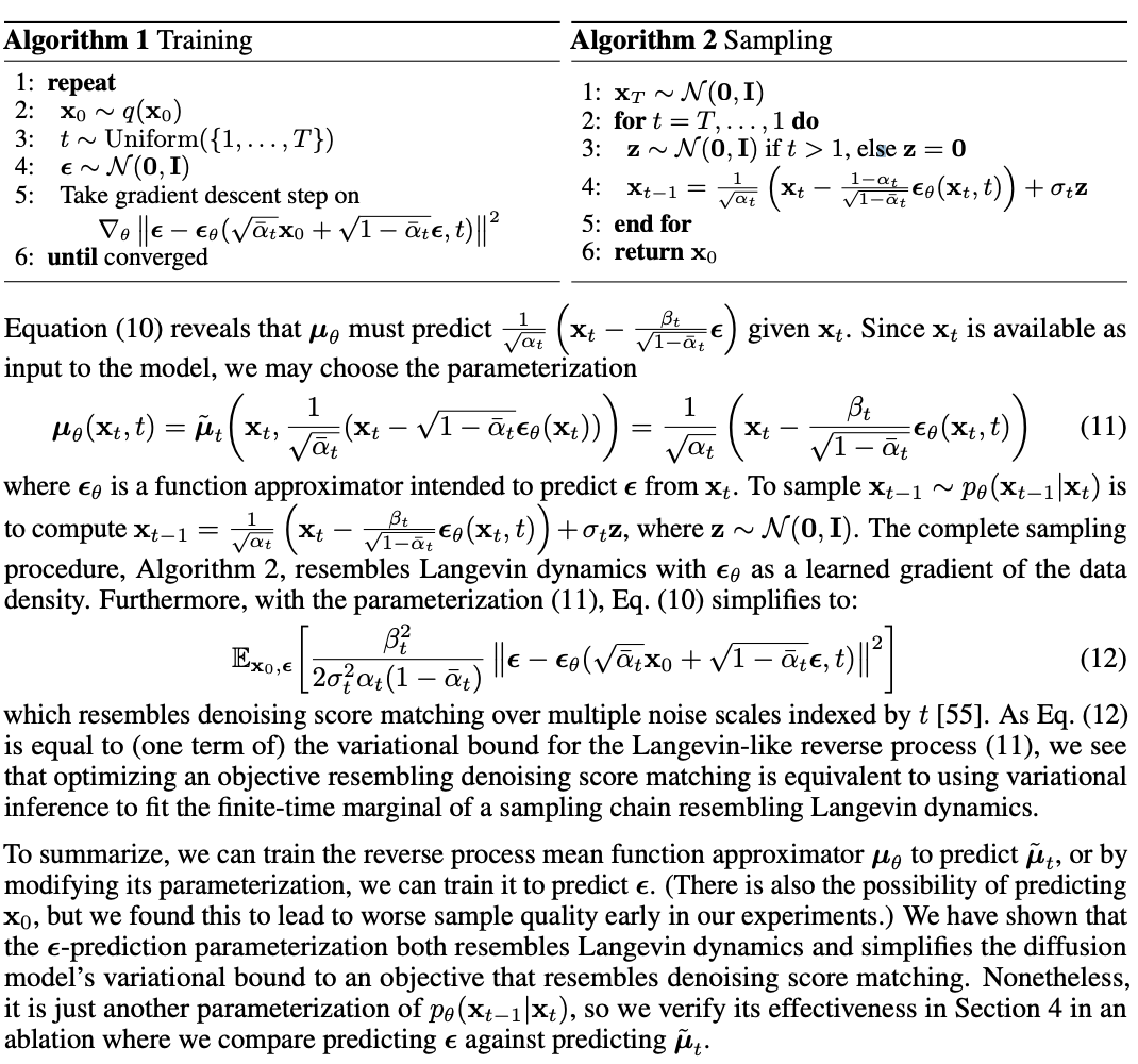
(12)에서 계수가 1일경우가 실험적으로 좋은 결과를 나타낸다고 하여서 계수를 1로 설정하였고 DDPM에서 제시한 Diffusion Model의 Loss식은 다음과 같다.

$q(x_t|x_{t-1}) = \mathcal{N}(x_t; \sqrt{\alpha_{t}}x_{t-1}, (1-\alpha_t)\mathcal{I})$
$p_{\theta}(x_{t-1}|x_t) := \mathcal{N}(\mu_{\theta}(x_t), \sum_{\theta}(x_t))$