[Paper Review] DDIM(Denoising Diffusion Implicit Models)
DDIM
- Paper: Denoising Diffusion Implicit Models ; arxiv
Introduction
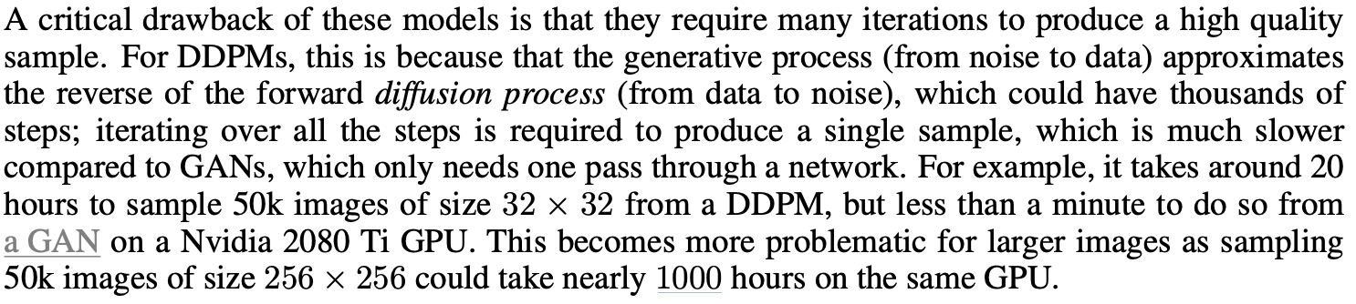
기존 DDPM에서는 reverse step을 설계했다기 보다는 forward process에서 어떤 식으로 noise를 주입할지 먼저 정한 후 forward process의 식으로 부터 denoising step을 bayes rule을 통해 유도하여서 이용하였다. Markov chain 특성을 사용해서 Forward, Reverse process를 모두 설계하였는데 이로 인해 Sampling시 모든 time step T를 거쳐서 원본이미지를 inference해야 하기에 시간이 너무 오래 걸리는 단점이 있다. 실제 DDIM논문에서도 이에 대해 언급하였다.
이번 논문에서는 기존 DDPM의 학습 방법은 그대로 가져가면서 markov chain 특성을 끊고 non-markov chain 특성을 이용해 더 빠르게 sampling 하면서 동시에 좋은 quality를 가져가는 방법에 대해서 제시한다.
BackGround
DDPM에서 제시했던 식들에 대해 알아보는 과정이다.
Denoising Network p에 대한 marginal, joint distribution을 나타내면 다음과같다.

$q(x_0)$를 알고 있을 때, denoising network p는 $p_{\theta}(x_0)$는 $q(x_0)$를 모사하기 위해 학습한다. 그리고 intractable한 $log(p_{\theta}(x_0))$를 해결하기 위해 ELBO를 이용하여 Objective Function을 도출했고 이는 다음과 같다.
$\underset{\theta}{max} \mathbb{E_{q(x_0)}}[p_{\theta}(x_0)] \le \underset{\theta}{max} \mathbb{E_{q(x_0), q_(x_1), \dots, q_(x_T) }}[log(p_{\theta}(x_{0:T})) - log(q(x_{1:T}|x_0))]$
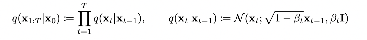
noise를 더하는 과정인 forward process는 markov chain성질에 의해 이루어지고 trainable하지 않고 fixed된 과정이다. 미리 scheduling 되어 있는 $\alpha_{1:T} \in (0,1]^T$에 의해 forward process는 다음과 같이 나타낼 수 있다.
위 식을 reparemeterization trick을 이용해 나타내고 $x_{t-1}, x_{t-2}, \dots, x_0$에 대해 점진적으로 나타내면 $x_t$는 다음과 같이 정리된다.
$x_t = \sqrt{\bar\alpha_{t}}x_0 + \sqrt{1-\bar\alpha_{t}}\epsilon$ ($\bar\alpha_{t} = \prod_{i=1}^{T}\alpha_i$), where $\epsilon \sim \mathcal{N}(0,\mathcal{I})$
그리고 Loss function은 다음과 같이 나타낸다.
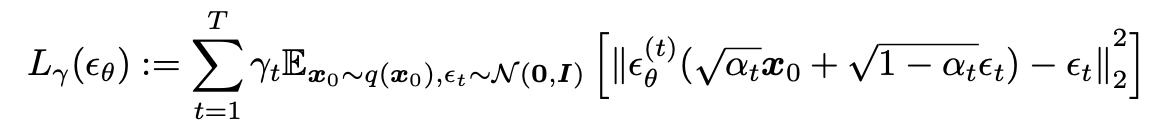
$\gamma_t$의 값이 1일 때 training model에 대한 generation performance가 최대가 된다고 하여서 $\gamma_t$의 값은 1로 설정하였다.
Variational Inference For Non-Markovian Forward Process
3.1 Non-Markovian Forward Process
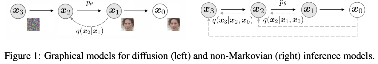
Generative Process는 inference process의 역과정으로 이루어진다. 생성 속도를 향상 시키기 위해서는 iteration을 줄여야 하기에 이를 위한 inference process를 다시 생각해봐야 한다. DDPM에서 Loss식을 보면 marginal distribution $q(x_{T}|x_0)$에만 의존하고, joint distribution인 $q(x_{1:T}|x_0)$에는 의존하지 않는다. 같은 marginal distribution을 가지는 수많은 joint distribution(inference process)가 존재하기에 새로운 inference process를 탐구해볼 수 있다.
$\boxed {q_{\sigma}(x_{1:T}|x_0) := q_{\sigma}(x_T|x_0) \prod_{t=2}^{T} q_{\sigma}(x_{t-1}|x_t,x_0) }$
증명)
$\prod_{t=1}^{T} q_{\sigma}(x_t|x_{t-1},x_0) = q_{\sigma}(x_1|x_0) \times q_{\sigma}(x_2|x_1,x_0) \times \dots \times q_{\sigma}(x_T|x_{T-1},x_0)$ $q_{\sigma}(x_t|x_{t-1},x_0) = \cfrac{q_{\sigma}(x_{t-1}|x_t,x_0) q_{\sigma}(x_t|x_0)}{q_{\sigma}(x_{t-1}|x_0)}$이기에$\prod_{t=1}^{T} q_{\sigma}(x_t|x_{t-1},x_0) = q_{\sigma}(x_1|x_0) \times \cfrac{q_{\sigma}(x_{1}|x_2,x_0) q_{\sigma}(x_2|x_0)}{q_{\sigma}(x_{1}|x_0)} \times \cfrac{q_{\sigma}(x_{2}|x_3,x_0) q_{\sigma}(x_3|x_0)}{q_{\sigma}(x_{2}|x_0)} \times \dots \times \cfrac{q_{\sigma}(x_{T-1}|x_T,x_0) q_{\sigma}(x_T|x_0)}{q_{\sigma}(x_{T-1}|x_0)}$
$= q_{\sigma}(x_T|x_0) \prod_{t=2}^{T} q_{\sigma}(x_{t-1}|x_t,x_0)$
$\boxed{ q_{\sigma}(x_{t-1}|x_t, x_0) = \mathcal{N}(\sqrt{\bar\alpha_{t-1}}x_0 + \sqrt{1- \bar\alpha_{t-1} - \sigma^2}\cfrac{x_t - \sqrt{\bar\alpha_t}x_0}{\sqrt{1-\bar\alpha_t}}, \sigma^2\mathcal{I}) }$
증명)
$x_{t-1} = \sqrt{\bar\alpha_{t-1}}x_0 + \sqrt{1-\bar\alpha_{t-1}}\epsilon_{t-1}$$x_{t-1} = \sqrt{\bar\alpha_{t-1}}x_0 + \sqrt{1-\bar\alpha_{t-1}-\sigma^2}\epsilon_{t} + \sigma\epsilon_t$(reparameterization trick)
$x_{t-1} = \sqrt{\bar\alpha_{t-1}}x_0 + \sqrt{1-\bar\alpha_{t-1}-\sigma^2}\cfrac{x_t - \sqrt{\bar\alpha_t}x_0}{\sqrt{1-\bar\alpha_t}} + \sigma\epsilon_t (x_t = \sqrt{\bar\alpha_{t}}x_0 + \sqrt{1-\bar\alpha_{t}}\epsilon_t$)
=> $\sigma$값에 따라 forward process가 얼마나 stochastic한지 정할 수 있으며, $\sigma$값이 0인 경우에는 $x_0, x_t$값이 주어졌을 때 $x_{t-1}$값이 deterministic하게 정해지는 극단적인 경우가 설정된다.
3.2 Generative Process and Unified Variational Inference Objective
Denoising Network p가 Generate Process를 거치는 방법은 다음과 같다.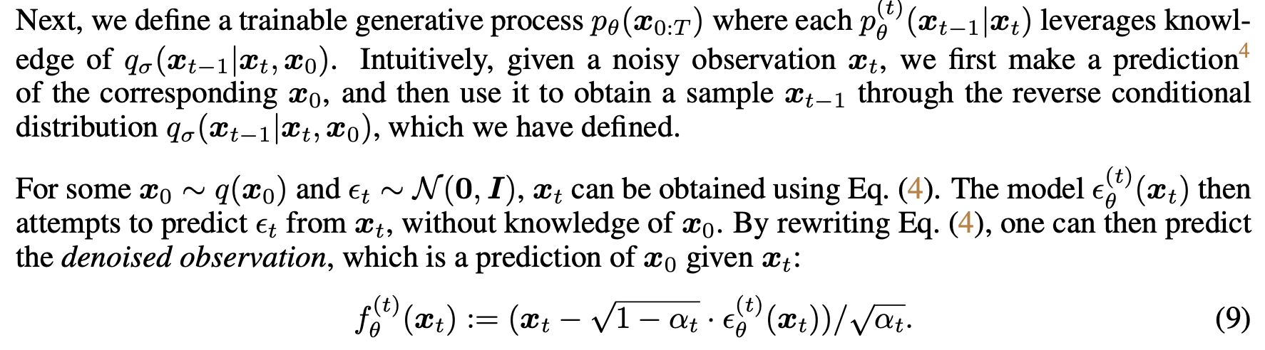
$x_t$가 주어졌을 때 Denoising Network $p_{\theta}$는 $x_t$로 부터 $\epsilon_t$를 예측한다. 예측한 $\epsilon_t$와 주어진 $x_t$를 통해 $x_0$를 예측할 수 있게 된다. $x_t, x_0$가 주어졌기에 $q_{\sigma}(x_{t-1}|x_t,x_0)$에 따라 $x_{t-1}$을 예측한다.
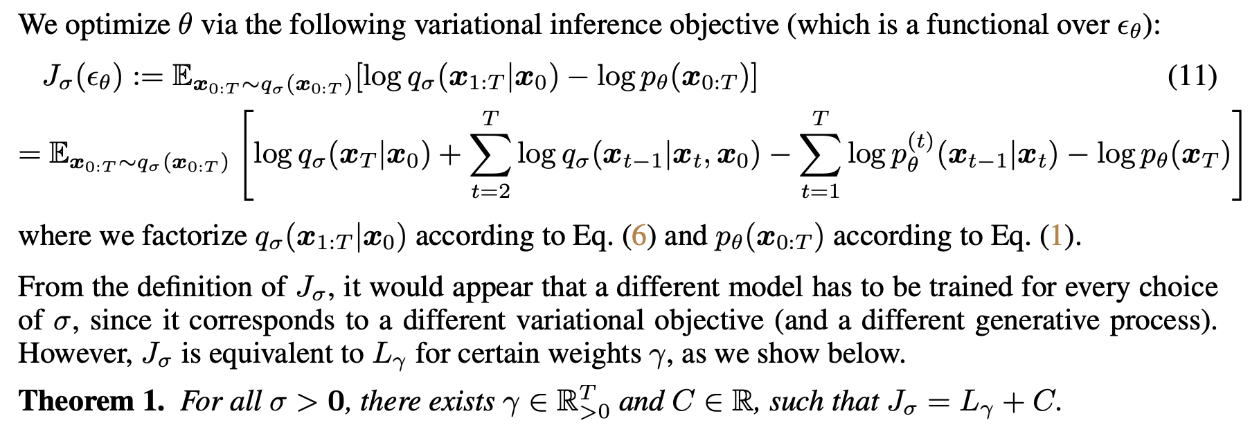
$\sigma$를 어떻게 설정하느냐에 따라 목적함수가 달라져서 서로 다른 모델이 필요하다.
- $\sigma = 0$이면, 위의 함수는 DDIM의 Loss Function이 된다.
- $\sigma = 1$이면, 위의 함수는 DDPM의 Loss Function이 된다.
Variational objective $L_{\gamma}$의 특별한 점은 $\epsilon_t^{(\theta)}$가 서로 다른 t에 대해서 공유되지 않는다면, $\epsilon_t^{(\theta)}$의 최적해는 weight $\gamma$에 의존하지 않는다는 점이다. 이러한 특징은 두 가지 의미를 갖게 된다.
- $L_1$은 DDPM의 variational lower bound에 대한 대리 목적 함수로 사용할 수 있다.
- $J_{\sigma}$는 일부 $L_{\gamma}$와 같기 때문에, $J_{\sigma}$의 최적해를 $L_1$과 같다고 볼 수 있다.
4. Sampling From Generalized Generative Process
$L_1$ objective function으로 Markovian inference process(ex. DDPM)뿐만 아니라 Non-Markovian inference process(ex. DDIM)를 위한 generative process를 학습할 수 있다. 그러므로 pre-trained된 DDPM 모델을 새로운 objective function에 대한 solution으로 사용할 수 있고, 우리의 필요에 맞게 $\sigma$를 변형시켜 sampling을 더 잘하는 generative process를 찾을 수도 있다.
4.1 Denoising Diffusion Implicit Models
주어진 sample $x_t$로 부터 $x_{t-1}$을 구하는 식은 아래와 같다.
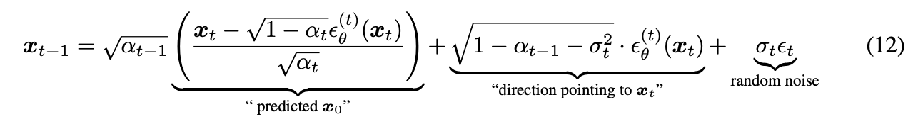
$\epsilon_t$ ~ $\mathcal{N}$(0, $\mathcal{I}$)는 $x_t$의 가우시안 noise이며 $\alpha_0 := 1$로 정의한다.
다른 $\sigma$를 사용하는 것은 다른 generative process를 만들지만, $\epsilon_{\theta}$를 이용하는 동일한 모델을 사용하기에 재학습은 불필요하다.
$\boxed{\sigma = \sqrt{(1-\bar\alpha_{t-1})/(1-\bar\alpha_t)}\sqrt{1-\alpha_t}}$, for all t
위의 식을 만족하면 forward process는 Markovian이 되며 generative process가 DDPM이 된다.
만약 $\sigma$ = 0이 되는 특별한 경우에는 forward process에서 noise를 더하는 항이 사라지므로 모든 step이 deterministic해지고 $x_T$부터 $x_0$까지 모두 고정된 샘플링 절차를 걸치기에 우리는 이 모델을 DDPM 목적함수로 학습이 된 Implicit한 모델이라고 부르며 이를 DDIM이라고 설정하였다.
4.2 Accelerated Generation Process
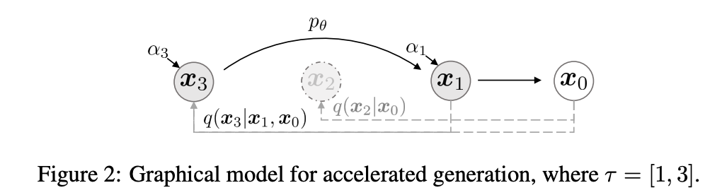
이전 까지만 하더라도 generative process는 reverse process에 대한 근사로 고려되었다. 따라서 forward process가 T step을 거쳐 이루어졌기에 generative process 역시 T step을 거치도록 설계되었다. 하지만 objective function L1에서는 marginal distribution인 $q_{\sigma}(x_t|x_0)$에만 의존을 하기에 forward process(joint distribution)와는 상관이 없었다. 따라서 T step보다 더 짧은 forward process도 고려할 수 있다.
forward process가 모든 latent variables $x_{1:T}$가 아니라 subset {$x_{\tau_1}, \dots, x_{\tau_S}$}라고 정의할 때,
$\tau$는 [1,$\dots$,T]의 증가하는 sub-sequence이며 $q(x_{\tau_i}|x_0) = \mathcal{N}(\sqrt{\alpha_{\tau_i}}x_0, (1-\alpha_{\tau_i}\mathcal{I}))$를 만족한다.
Generative Process는 reversed($\tau$)에 따라서 latent variables를 sample하고 이를 sampling-trajectory라고 부른다. sampling-trajectory의 길이가 T보다 작으면, sampling하는 과정에서 상당한 속도 향상을 얻을 수 있다.
4.3 Relevance To Neural ODEs
4.1에 언급한 식(12)에 따라 DDIM 반복을 다시 작성하면, 일반 미분 방정식(ODE)를 풀기 위한 오일러 적분과 유사성이 더욱 분명해진다고 한다. 이를 통해 충분한 discretization steps를 거치면, ODE를 reverse해서 encoding($x_0$ -> $x_T$)도 가능하다.